A simplification of Budyko's ice-albedo feedback model
Richard McGehee and Esther Widiasih
preprint (2012)
| School of Mathematics | |||||||||
| Richard McGehee | |||||||||
| |||||||||
| Abstract. A classical model of ice-albedo feedback was recently augmented to incorporate ice line dynamics, and the resulting infinite dimensional dynamical system was reduced to a one-dimensional system using invariant manifold theory. Here we introduce an approximation to the model, which immediately produces a five-dimensional dynamical system having an analogous one-dimensional invariant manifold. We derive a simple ordinary differential equation approximating the system and use it to estimate the value of a parameter left unspecified in previous work. |
|
Download Preprint (pdf) |
|
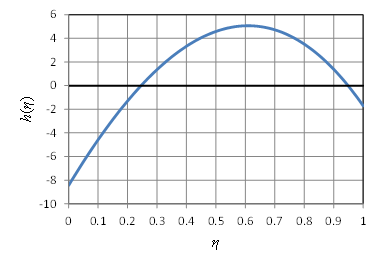
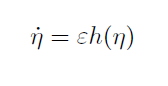
Description Albedo is the reflectivity of a surface, in this case, the surface of the Earth. Ice has a higher albedo than water and land. The feedback mechanism can be described as follows. If the ice is advancing, more of the Sun's energy is reflected from the surface, cooling the Earth and causing the ice to advance. If the ice is retreating, more of the Sun's energy is absorbed by the surface, warming the Earth and causing more ice to melt. Budyko's model offers an explanation for why the feedback reaches an equilibrium. The model can be written $$R\frac{\partial T}{\partial t} = Qs(y)(1-\alpha(y)) - (A+BT) + C(\overline{T}-T),$$ where \(T\) is the surface temperature as a function of \(y\), the sine of the latitude, and \(t\), time. The albedo \(\alpha\) is assumed to be a function of latitude. The outgoing long wave radiation is approximated linearly with the term $$A+BT.$$ The transfer of heat from warmer latitudes to colder is also approximated linearly with the term $$C(\overline{T} - T),$$ where \(\overline{T}\) is the annual average global temperature, given by $$\overline T = \int_0^1 T(y)dy.$$ The parameter \(R\) is the heat capacity of the Earth's surface. The planet is assumed to be covered with ice for latitudes above a value given by \(y=\eta\) and to be ice-free for values below that. Therefore we write $$\alpha(y) = \alpha(y,\eta) = \left\{ \begin{matrix} \alpha_1, & y < \eta , \\ \alpha_2, & y > \eta , \\ \end{matrix} \right.$$ where \(\alpha_1\) is the albedo of ice and \(\alpha_2\) is the albedo of ocean and land. Widiasih introduced the following equation for the dynamics of the ice line \(\eta\): $$\frac{d\eta}{dt} = \epsilon(T_b - T_c),$$ where \(T_b\) is the average temperature across the ice boundary, i.e., $$T_b = \frac{T(\eta -) + T(\eta +)}{2},$$ and where \(T_c\) is the critical annual mean temperature above which ice retreats and below which ice advances. This equation simply states that the movement of the ice line is proportional to the difference between the current temperature at the ice line and the critical temperature. The equation for the surface temperature \(T\) can be combined with the equation for the ice line \(\eta\) to form a single dynamical system with a state space consisting of the Cartesian product of the interval \([0,1]\) (the values of \(\eta\)) with a space of possible functions \(T(\eta)\). Taking this function space to be piecewise quadratic functions yields a five-dimensional dynamical system which approximates the original system. Using standard techniques, one finds that this system has a one-dimensional attracting invariant manifold, containing the essential long-term behavior of the system. On the invariant curve, the system is approximated by the single ordinary differential equation $$\frac{dh}{dt} = \epsilon h(\eta).$$ The graph of the function \(h\) for appropriate values of the parameters is shown below. One sees that there is a stable rest point at \(\eta\approx 0.95\) and an unstable one at \(\eta\approx 0.25\).
The function \(h\) can be written $$ h(\eta) = \Phi_0(\eta) + \frac{Qs_2(1-\alpha_0)}{B+C}\cdot\frac{3\eta^2 - 1}{2} - T_c\,, $$ where $$ \Phi_0(\eta) = \frac 1B \left( Q(1-\alpha_0) - A + C\frac{Q(\alpha_2 - \alpha_1)}{B+C} \left( \eta - \frac12 + s_2\frac{\eta^3 - \eta}{2} \right) \right).$$ Appropriate values of the parameters are given in the table below.
|