Math 5-385: Surface plot info

Math 5-385
Info about using Matlab for plotting surfaces in 3-space
with emphasis on parametric surfaces

Major update completed: December 12, 2008
Smaller updates done on December 15, 2008

Contents

The basics
Useful matrix commands
¡¡ New !! An improved approach to surface plotting
Manipulating the Matlab graphics window

Further specific examples As of Dec. 15, 2008 the sphere and torus examples have been updated,
but the snowcone example still is somewhat out of date.

The basics
In this section, we'll tell you how to get started, and point you toward the basic Matlab help page that explains how to do surface plots. After reading that, you probably can go directly to material on the improved approach to surface plotting. The section on useful matrix commands still includes valuable material, but it is not possible to do surface plots without understanding that material. And when you have a basic figure that you'd like to tweak, you may consul the section on manipulating the Matlab graphics window.

We begin by starting Matlab, as usual, from the Applications menu on the main Fedora (linux) screen. This will open two windows: [1] the command window (where you enter Matlab commands) and [2] the help window. The command window has a history sidebar, where you can look up commands that you've entered in previous sessions. {You can copy one or more of those old commands into the active command window if that seems like a good idea.} The help window presents a topical index, which you can navigate to find information about Matlab tools that you want to work with. {It does, however,take some practice to get used to the way that this is set up.}

Click to expand the "Matlab" heading in the left hand column of the Help window (right below "Release Notes" and "Installation". In this subsection (where the headings appear in blue) you can find a majority of the most relevant topics if you click to expand the "Graphics" and/or "3-D Visualization" headings.

Under this heading the following links will be particularly useful for us:

Representing a Matrix as a Surface. This section explains the idea of seting up a rectangular grid.
Parametric Surfaces. The examples that we'll be able to draw most effectively are surfaces that are presented parametrically. This section includes a nice example of how to sketch one of those.

At the very bottom of the left column there is a link called Plotting and Visualization Function. Clicking on this link produces an extensive list in the right column. That list, which includes links to help text for specific commands, includes most of the plotting commands that we're likely to need.

To find other useful commands including commands for working with matrices, go back to the main helpdesk window. Under the heading "MATLAB Functions" in the left column, the link "by Subject" usually is most effective. There are several useful links in the window that appears next, including Elementary Matrices and Matrix Multiplication and Operators and Special Characters. The latter list includes [for instance] an explanation of the very important difference between matrix multiplication, denoted * (as expected), and array (or elementwise) multiplication, which is denoted .* instead.

When finished remember to close the browser window. This will make things go a lot more smoothly the next time you run Netscape on the math department system.

Some useful matrix commands

To enter a matrix element by element:
>> >> A = [1 2; 0 -3] A = 1 2 0 -3 >> B = [-7 -9] B = -7 -9 >> C = [7 9]' C = 7 9
(The single quote stands for "transpose").

The following is just for practice:

>> >> C + B' ans = 0 0

Stacking two matrices side by side:
> >> [A C] ans = 1 2 7 0 -3 9
(Note that both must have the same number of rows).

Stacking one matrix on top of another:
>> >> [A; B] ans = 1 2 0 -3 -7 -9
(Here, they must have the same number of columns).

Building a matrix from several blocks:
>> >> [A C; B 0] ans = 1 2 7 0 -3 9 -7 -9 0

Maybe we were lucky, since we didn't tell MATLAB the size of
the matrix of zeros. But we can create a matrix of zeros
of any specified size:
>> >> zeros(4,2) ans = 0 0 0 0 0 0 0 0
Similarly, if we want a matrix of ones:
>> >> ones(3,5) ans = 1 1 1 1 1 1 1 1 1 1 1 1 1 1 1
Of course, we also have identity matrices:
>> >> eye(3) ans = 1 0 0 0 1 0 0 0 1

Matrix multiplication, exponentiation, and inverse commands in MATLAB:

Let's recall some of our earlier matrices:
>> >> A A = 1 2 0 -3 >> B B = -7 -9 >> C C = 7 9
Now, for the operations:
>> >> A*C ans = 25 -27 >> B*A ans = -7 13 >> A^2 ans = 1 -4 0 9 >> A^-1 ans = 1.0000 0.6667 0 -0.3333

We also can do componentwise operations.

Raising all entries of a matrix to a fixed power:
>> >> A.^3 ans = 1 8 0 -27 >> B.^2 ans = 49 81
Multiplying the elements of one matrix by the corresponding
elements of another matrix. In the MATLAB help pages,
this is called array multiplication.
>> >> B.*C ??? Error using ==> .* Matrix dimensions must agree. >>
Since B is 1 by 2 and C is 2 by 1, we had better use one of the transposes: >> >> B.*C' ans = -49 -81
One other thing: to apply a function to all of the entries of a matrix,
just substitute the matrix into the function command: >> >> sin(pi*(0:1:24)/12) ans = Columns 1 through 7 0 0.2588 0.5000 0.7071 0.8660 0.9659 1.0000 Columns 8 through 14 0.9659 0.8660 0.7071 0.5000 0.2588 0.0000 -0.2588 Columns 15 through 21 -0.5000 -0.7071 -0.8660 -0.9659 -1.0000 -0.9659 -0.8660 Columns 22 through 25 -0.7071 -0.5000 -0.2588 -0.0000

An improved approach to surface plotting (under construction as of December 10, 2008)

As usual, the goal is to draw a surface which is given parametrically:

x = f(t,u)
y = g(t,u)
z = h(t,u), where the variables range through some specific intervals, say a ≤ t ≤ b, c ≤ u ≤ d.
As a specific instance, let's consider the Whitney umbrella surface (see exercise 9 in sec 3.3).
Thus, f(t,u) = t, g(t,u) = u², and h(t,u) = tu, so that: x = t
y = u²
z = tu, where -1 ≤ t ≤ 1 and -1 ≤ u ≤ 1.

Step 1: enter the functions. Here, we use the standard computer notation for math operations
such as multiplication and exponentiation. f = 't' g = 'u^2' h = 't*u' Note: The single quotes are very important.
Step 2: convert the functions to vector form. F = vectorize(f) G = vectorize(g) H = vectorize(h)
If you've entered it like this, omitting the semicolon at the end of the line, then Matlab will show you the output. For the last two commands, it will look something like this: G = u.^2 H = t.*u The explanation here is that the strings .^ and .* are Matlab's notation for componentwise exponentiation of a matrix and componentwise multiplication of two matrices of the same size. And very shortly, after creating matrix values for the variables t and u, we will evaluate the functions F, G, H to assign them matrix values.
Step 3: Create matrix values for the variables.
- Part a: establish divisions in the t and u intervals. Here, we'll just divide each of the intervals, running from -1 to +1, into subintervals of length 0.1. But you don't have to divide them into equal numbers of subintervals. You can use a lot more subintervals if greater smoothness is desirable, while considerably few subintervals sometimes may be desirable (for instance when dealing with a surface which is a union of continuously varying straight lines). r = -1:0.1:1; s = -1:0.1:1; The output of each command is a row vector with 21 entries. We probably don't want to look at it on the screen, so we put a semicolon at the end of the command line in order to hide the output.
- Part b: use these row vectors to create the desired matrix values. [t,u] = meshgrid(r,s); The output here will be two matrices of size 21 by 21, one of them for t and the other for u. If we don't want to look at those matrices, we put the usual semicolon at the end of the row. But it may be worth mentioning that the t-matrix has constant columns and the u-matrix has constant rows. {I checked this by looking at the output from a 5 by 5 example.}
Step 4: Evaluate the functions F, G, H to get matrix values for the coordinates. X = eval(F); Y = eval(G); Z = eval(H);
Step 5: (¡¡finally!!) draw the surface. S = surf(X,Y,Z);
This produces the following image:
Step 5 variant: draw a mesh which shows how the gridlines in the tu-plane are mapped to curves on the surface: M = mesh(X,Y,Z);
(The result is not shown here.)

Manipulating the Matlab graphics window

We'll look at the previous surface, i.e. the Whitney umbrella surface, to see specific examples of things that can be done. First of all, since t occurs only to the first power in the parametrization, our surface is a ruled surface. This means that it is a union of straight lines. To show this more clearly, we will change the grid so that the u-interval has divisions only at -1, 0, and 1. And (skipping a step that was done in class), we'll also combine this with dividing the t interval into 20 subintervals instead of 10. 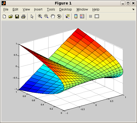We keep the functions f, g, h and the vectorized functions F, G, H as before, and just re-calculate the steps that need to be changed: r = [-1 0 1]; s = -1:0.05:1; [t,u] = meshgrid(r,s); X = eval(F); Y = eval(G); Z = eval(H); S = surf(X,Y,Z); This time we get the following figure:

This has some desirable features, but the color of the right half is disappointing. This is related to the default values that Matlab uses in calculating the color data. We can, however, use Matlab's set to substitute a matrix of our own choice for the color data. This matrix must be of the same size as the X, Y or Z matrices in the plot. For our ruled surface, the u matrix is a good choice, because the lines on the surface correspond to u-values. Accordingly, here is an appropriate command: set(S,'CData',u) Here is the result:

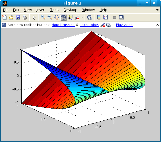
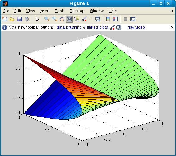
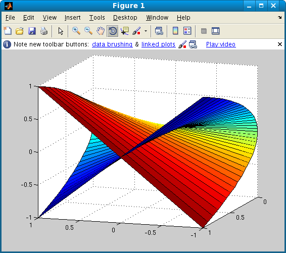
Now, it might be nice to see the surface from a different direction. To accomplish that, we click on the rotate icon

on the toolbar and then use the mouse to rotate the figure. Among many other possibilities, here is one position to which it can be moved:

Here are some other things that you can do:

From the Insert menu:
- Add a title, a text box (including explanations, etc.), axis labels, or a legend, among other possibilities.
From the Edit menu:
- Select the main figure, or one of the things added above, and then choose Current object properties from the menu.
From the File menu:
- Select Save to save your figure as a Matlab figure, or choose Save as ... to save the image as a .jpeg file, among other possibilities.
Click on the rotate icon and then use the mouse to rotate your figure.
Click on the zoom in icon and then click on the figure to zoom in.
Click on the zoom out icon and then click on the figure to zoom out.
Click on the edit icon and then use various tools to add features to your figure.
Use the set command {from the main Matlab window} to change lineWidth, or lineStyle, or some other aspects. Among other possibilities, 'none' is a valid line style, so that we even can remove the lines completely and exhibit a smooth surface.
- We can make the lines a bit heavier, if we wish:
  
  set(S, 'linewidth',2)
- On the other hand, if we'd like to get rid of the gridlines on the surface, then we can use the following command:
  set(S, 'linestyle','none')
- If we didn't like the result of that last move, and would like to restore the solid line, then we can do the following:
  set(S, 'linestyle','-')

Further specific examples and sugestions
Although the first two examples below are given by trigonometric parametrizations, they're actually algebraic surfaces -- the first one obviously so, because of its well known equation x² + y² + z² = 1.
Any of the matlab text presented below can be copied from this window and pasted into a Matlab command window. If desired, you can then modify it to plot other figures.

The sphere
Here is a sequence of Matlab commands which produces the drawing of the unit sphere shown below.
The small rectangles in the grid are squares in which the length of the side is  π/24.

f = 'sin(phi)*cos(theta)' g = 'sin(phi)*sin(theta)' h = 'cos(phi)' F = vectorize(f) G = vectorize(g) H = vectorize(h)        %Our functions are now in the form that Matlab will need. r = pi*(-24:1:24)/24;        %This gives a row vector (1 by 49). s = pi*(0:1:24)/24;         %This also gives a column vector (25 by 1). [theta,phi] = meshgrid(r,s);     %This gives theta and phi as 25 by 49 matrices. X = eval(F); Y = eval(G); Z = eval(H);        %These commands evaluate our functions at the gridpoints.                      The results are stored as 25 by 49 matrices. surf(X,Y,Z)

With the default settings, this produces a somewhat flattened looking sphere. Click here if you would like to see it. We can use a fairly easy matlab command to get a more symmetric sphere, namely:

       axis square

Here is the final result:

Some comments:

The semicolons at the ends of the lines suppress the output.
So, the matrices don't appear on our computer screen.
(But we don't need semicolon in the line that produces the graphics window ... )
The expression (-24:1:24) produces a row vector whose entries range from -24 to 24 in steps of 1.
The commands sin and cos (as well as other basic math functions) act entry by entry on a matrix.
The asterisk * produces the usual matrix product, while the string .* multiplies each entry of one matrix by the corresponding entry of another matrix of the same size. (This operation is called componentwise multiplication.)
We are accepting the default color map, in which points on the surface are colored according to their z-coordinates.
The torus
The mathematical aspects here are relatively standard; this example also exhibits a method of manipulating the graphics window to produce aobetter sketch. The torus that we will plot is obtained by rotating (about the z-axis) the circle in the yz-plane with center (0,2,0) and radius 1, as shown in the figure.


So, the z-coordinate of a point on the circle is given by the formula z = sin(φ), and its distance from the z-axis (equal to the y-coordinate in this cross section is given by the formula r = 2 + cos(φ). If we describe our torus parametrically in cylindrical coordinates, it is then given as follows:

x = (2 + cos(φ))cos(θ),     y = (2 + cos(φ))sin(θ),     z = sin(φ). Therefore, the following sequence of commands will produce a Matlab plot of our torus:

r = pi*(-24:1:24)/24; s = pi*(-24:1:24)/24; [theta phi] = meshgrid(r,s); f = '(2 + cos(phi))*cos(theta)'; g = '(2 + cos(phi))*sin(theta)'; h = 'sin(phi)'; F = vectorize(f); G = vectorize(g); H = vectorize(h); x = eval(F); y = eval(G); z = eval(H); surf(x,y,z)
Here's what this produces:



The figure is literally correct, but the scales for the various axes (the defaults chosen by Matlab) make the figure look out of proportion. The "cheapest" way to fix this is by changing the size of the graphics window -- just grab the lower right corner with the mouse, using the left button. Click here to see a (slightly cropped) picture of what we can accomplish in this way. Alternatively, we can get a similar (but somewhat smaller) result by using the Matlab command    axis square

Another way to fix the scaling problem is by editing the axes properties, found under the Tools menu at the top of the graphics window. For instance, if the x and y limits are set to run from -3 to 3, and the z limits are set to run from -1.5 to 1.5, then we get a pretty credible sketch with the original window size. [To change any number in the dialog box, click the corresponding "manual" button.] To see the result of this process, click here.
The "snow cone"
Sometimes a picture of a surface has to be drawn in two pieces because various parts are described by different parametric formulas. That's the case here, since one part is a portion of a sphere while the other part is a portion of a cone. So, this example shows the use of the Matlab command "hold on", which makes it possible for previously drawn parts of the picture to remain while new parts are added. (If you make a mistake, then the command "hold off" makes it possible to start over.)

We use spherical coordinates, by means of the usual formulas:

x = ρ sin(φ) cos(θ), y = ρ sin(φ) sin(θ), z = ρ cos(φ),

and we begin by drawing a cone, such that a generating line segment has length = 1 and makes an angle of π / 6 radians with the positive z-axis. Therefore, φ has a constant value, namely π / 6. We'll approximate the cone with triangular pieces with one vertex at the origin, but they're actually drawn as rectangles, with two vertices at the origin. So, here's a series of Matlab commands that will implement this:

theta = (0:1:36)*pi/18; rho = [0 1]'; x = rho*cos(theta)*sin(pi/6); y = rho*sin(theta)*sin(pi/6); z = rho*ones(size(theta))*cos(pi/6); cone = surf(x,y,z); axis square
The resulting picture has a fairly monotonous coloring, but we can vary the color in a fairly nice way by using a new matrix of color data:

c1 = [1 1]'*cos(theta); set(cone,'CData',c1)

Now, we "freeze" the picture so that new material can be added:

hold on
The next order of business is to draw an appropriate piece of spherical surface on top of the cone. This time, it is ρ that has a constant value, namely ρ = 1. So, we simply leave rho out of the formulas.

phi = (0:1:6)'*pi/36; X = sin(phi)*cos(theta); Y = sin(phi)*sin(theta); Z = cos(phi)*ones(size(theta)); cap = surf(X,Y,Z);

Now, we change the color data. (This step may be considered optional.) Note that our color data matrix has the same size as the matrices that defined the coordinates. Thus, we're actually telling Matlab what color each of the little patches has to be. Here, we're matching the color at the edge to the cone colors, and letting the color get a bit lighter as we move to the center of the cap.

c2 = (2:1:8)'*cos(theta)/8; set(cap,'CData',c2) To finish, we'll change the viewing angle slightly to make the spherical cap make a bit more rounded. The following command sets the azimuth (horizontal rotation) equal to -37.5 degrees and sets the elevation to 20 degrees.

view(-37.5,20)

For more information from inside Matlab, type help view

Here is the final result:

For more information. On the Matlab help page (type helpdesk at the Matlab prompt)
see the following items under the MATLAB topics menu:

To getting started for info about basic matrix commands, and related stuff
Using MATLAB graphics for info about surface plotting and other graphics topics
(In the new table of contents that comes up, scroll down a ways to find Creating 3-D Graphs.
Under that topic, there's a special link about Parametric Surfaces.).
Handle Graphics Properties for info about properties of graphics objects. There are commands for changing
many of these from the Matlab command window. For instance, with the surface example above, we can type:
set(S,'meshstyle','column') This gives us lines in just 1 direction, rather than a grid. Another version
is: set(S,'meshstyle','column')To get the grid back, type >> set(S,'meshstyle','both')
Changing colors is also possible, but somewhat more elaborate.
MATLAB functions There are links to an index and to a list organized by topics

Comments and questions to: roberts@math.umn.edu

Back to the help page index.

Back to the Math 5385 class homepage.