Periodic Table of the Finite Elements
Background
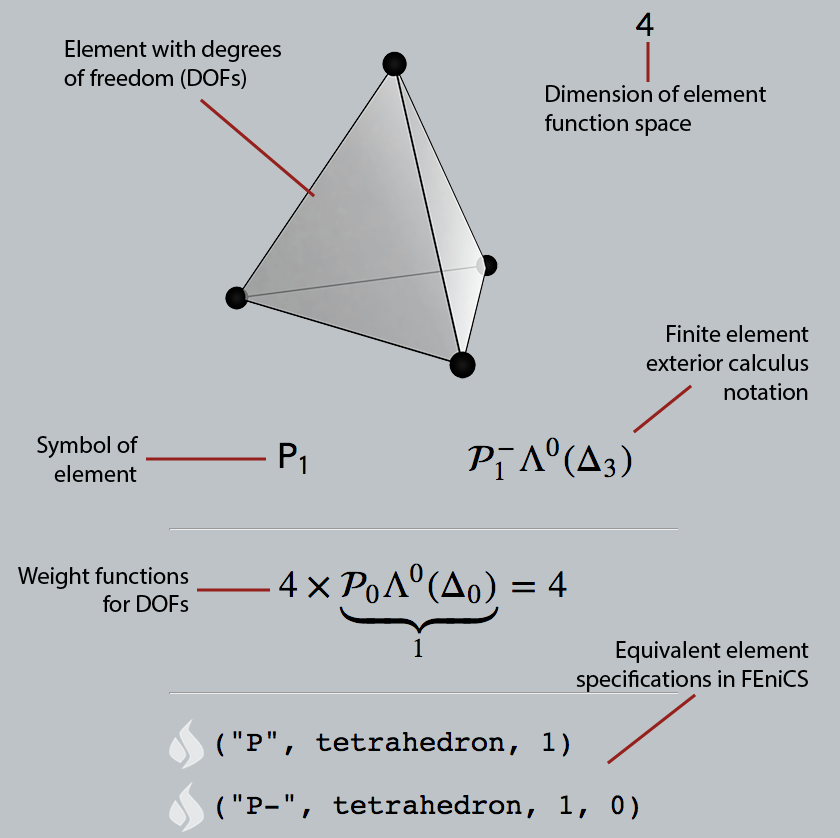
The table presents the primary spaces of finite elements for the discretization of the fundamental operators of vector calculus: the gradient, curl, and divergence. A finite element space is a space of piecewise polynomial functions on a domain determined by: (1) a mesh of the domain into polyhedral cells called elements, (2) a finite dimensional space of polynomial functions on each element called the shape functions, and (3) a unisolvent set of functionals on the shape functions of each element called degrees of freedom (DOFs), each DOF being associated to a (generalized) face of the element, and specifying a quantity which takes a single value for all elements sharing the face. The element diagrams depict the DOFs and their association to faces.
The spaces $\mP_r^-\Lambda^k$ and $\mP_r\Lambda^k$ depicted on the left half of the table are the two primary families of finite element spaces for meshes of simplices, and the spaces $\mQ_r^-\Lambda^k$ and $\mS_r\Lambda^k$ on the right side are for meshes of cubes or boxes. Each is defined in any dimension $n\ge 1$, for each value of the polynomial degree $r\ge 1$, and each value of $0 \leq k \leq n$. The parameter $k$ refers to the operator: the spaces belong to the domain of the $k$th exterior derivative. Thus for $k=0$, the spaces discretize the Sobolev space $H^1$, the domain of the gradient operator; for $k=1$, they discretize $H(\curl)$, the domain of the curl; for $k=n-1$ they discretize $H(\div)$, the domain of the divergence; and for $k=n$, they discretize $L^2$.
The spaces $\mP_r^-\Lambda^0$ and $\mP_r\Lambda^0$, which coincide, are the earliest finite elements, going back in the case $r=1$ of linear elements to Courant,1 and collectively referred to as the Lagrange elements. The spaces $\mP_{r+1}^-\Lambda^n$ and $\mP_r\Lambda^n$, which also coincide, are the discontinuous Galerkin elements, consisting of piecewise polynomials with no interelement continuity imposed, first introduced by Reed and Hill.2 The space $\mP_r^-\Lambda^1$ in 2 dimensions was introduced by Raviart and Thomas3 and generalized to the 3-dimensional spaces $\mP_r^-\Lambda^1$ and $\mP_r^-\Lambda^2$ by Nédélec,4 while $\mP_r\Lambda^1$ is due to Brezzi, Douglas, and Marini5 in 2 dimensions, its generalization to 3 dimensions again due to Nédélec.6 The unified treatment and notation of the $\mP_r^-\Lambda^k$ and $\mP_r\Lambda^k$ families is due to Arnold, Falk, and Winther as part of finite element exterior calculus,7 extending the earlier work of Hiptmair for the $\mP_r^-\Lambda^k$ family.8 The space $\mP_1^-\Lambda^k$ is the span of the elementary forms introduced by Whitney.9
The family $\mQ_r^-\Lambda^k$ of cubical elements can be derived from the 1-dimensional Lagrange and discontinuous Galerkin elements by a tensor product construction detailed by Arnold, Boffi, and Bonizzoni,10 but for the most part were presented individually along with the corresponding simplicial elements in the papers mentioned. The second cubical family $\mS_r\Lambda^k$ is due to Arnold and Awanou.11
The finite elements in this table have been implemented as part of the FEniCS Project12, 13, 14 Each may be referenced by the Unified Form Language (UFL)15 by giving its family, shape and degree, with the family as shown on the table. For example, the space $\P{3}{1}{3}$ may be referred in UFL as:
FiniteElement("N2E", tetrahedron, 3)
Alternatively, the elements may be accessed in a uniform fashion as:
FiniteElement("P-", shape, r, k)
FiniteElement("P", shape, r, k)
FiniteElement("Q-", shape, r, k)
FiniteElement("S", shape, r, k)
for $\mP_r^-\Lambda^k$, $\mP_r\Lambda^k$, $\mQ_r^-\Lambda^k$, and $\mS_r\Lambda^k$, respectively.
The $\mP_r^-\Lambda^k$ family
The shape function space for $\mP_r^-\Lambda^k$ is $\mP_{r-1}\Lambda^k+\kappa\mP_{r-1}\Lambda^{k+1}$ where $\kappa$ is the Koszul differential.7 It includes the full polynomial space $\mP_{r-1}\Lambda^k$, is included in $\mP_r\Lambda^k$, and has dimension
$$\dim \mP_r^-\Lambda^k(\Delta_n)=\binom{r+n}{r+k}\binom{r+k-1}{k}.$$
The degrees of freedom are given on faces $f$ of dimension $d\ge k$ by moments of the trace weighted by a full polynomial space:
$$u\mapsto \int_f (\tr_f u)\wedge q, \quad q\in\mP_{r+k-d-1}\Lambda^{d-k}(f).$$
The spaces with constant degree $r$ form a complex:
$$\mP_r^-\Lambda^0\xrightarrow{\mathrm d}\mP_r^-\Lambda^1\xrightarrow{\mathrm d}\cdots\xrightarrow{\mathrm d}\mP_r^-\Lambda^n.$$
| n | k | r = 1 | 2 | 3 | 4 | 5 | 6 | 7 |
|---|---|---|---|---|---|---|---|---|
| 1 | 0 | 2 | 3 | 4 | 5 | 6 | 7 | 8 |
| 1 | 1 | 2 | 3 | 4 | 5 | 6 | 7 | |
| 2 | 0 | 3 | 6 | 10 | 15 | 21 | 28 | 36 |
| 1 | 3 | 8 | 15 | 24 | 35 | 48 | 63 | |
| 2 | 1 | 3 | 6 | 10 | 15 | 21 | 28 | |
| 3 | 0 | 4 | 10 | 20 | 35 | 56 | 84 | 120 |
| 1 | 6 | 20 | 45 | 84 | 140 | 216 | 315 | |
| 2 | 4 | 15 | 36 | 70 | 120 | 189 | 280 | |
| 3 | 1 | 4 | 10 | 20 | 35 | 56 | 84 | |
| 4 | 0 | 5 | 15 | 35 | 70 | 126 | 210 | 330 |
| 1 | 10 | 40 | 105 | 224 | 420 | 720 | 1155 | |
| 2 | 10 | 45 | 126 | 280 | 540 | 945 | 1540 | |
| 3 | 5 | 24 | 70 | 160 | 315 | 560 | 924 | |
| 4 | 1 | 5 | 15 | 35 | 70 | 126 | 210 |
The $\mP_r\Lambda^k$ family
The shape function space for $\mP_r\Lambda^k$ consists of all differential $k$-forms with polynomial coefficients of degree at most $r$, and has dimension
$$\dim \mP_r\Lambda^k(\Delta_n)=\binom{r+n}{r+k}\binom{r+k}{k}.$$
The degrees of freedom are given on faces $f$ of dimension $d\ge k$ by moments of the trace weighted by a $\mP_r^-$ space:
$$u\mapsto \int_f (\tr_f u)\wedge q, \quad q\in\mP^-_{r+k-d}\Lambda^{d-k}(f).$$
The spaces with decreasing degree $r$ form a complex:
$$\mP_r\Lambda^0\xrightarrow{\mathrm d}\mP_{r-1}\Lambda^1\xrightarrow{\mathrm d}\cdots\xrightarrow{\mathrm d}\mP_{r-n}\Lambda^n.$$
| n | k | r = 1 | 2 | 3 | 4 | 5 | 6 | 7 |
|---|---|---|---|---|---|---|---|---|
| 1 | 0 | 2 | 3 | 4 | 5 | 6 | 7 | 8 |
| 1 | 2 | 3 | 4 | 5 | 6 | 7 | 8 | |
| 2 | 0 | 3 | 6 | 10 | 15 | 21 | 28 | 36 |
| 1 | 6 | 12 | 20 | 30 | 42 | 56 | 72 | |
| 2 | 3 | 6 | 10 | 15 | 21 | 28 | 36 | |
| 3 | 0 | 4 | 10 | 20 | 35 | 56 | 84 | 120 |
| 1 | 12 | 30 | 60 | 105 | 168 | 252 | 360 | |
| 2 | 12 | 30 | 60 | 105 | 168 | 252 | 360 | |
| 3 | 4 | 10 | 20 | 35 | 56 | 84 | 120 | |
| 4 | 0 | 5 | 15 | 35 | 70 | 126 | 210 | 330 |
| 1 | 20 | 60 | 140 | 280 | 504 | 840 | 1320 | |
| 2 | 30 | 90 | 210 | 420 | 756 | 1260 | 1980 | |
| 3 | 20 | 60 | 140 | 280 | 504 | 840 | 1320 | |
| 4 | 5 | 15 | 35 | 70 | 126 | 210 | 330 |
The $\mQ_r^-\Lambda^k$ family
This family is constructed from the complex of 1-dimensional finite elements using a tensor product construction.10 The shape function space on the unit cube $\square_n=I^n$ is given by
$$\mQ_r^-\Lambda^k(\square_n) = \bigoplus_{\sigma\in \Sigma(k,n)}\left[\bigotimes_{i=1}^n \mP_{r-\delta_{i,\sigma}}(I)\right]\, \mathrm{d}x^{\sigma_1}\wedge\cdots\wedge \mathrm{d}x^{\sigma_k}, $$
where $\Sigma(k,n)$ denotes the increasing maps $\{1,\ldots,k\}\to\{1,\ldots,n\}$. Its dimension is $\dim \mQ_r^-\Lambda^k(\square_n) =\binom{n}{k}r^k(r+1)^{n-k}. $ The degrees of freedom are
$$u \mapsto \int_f (\tr_f u)\wedge q, \quad q\in \mQ_{r-1}^-\Lambda^{d-k}(f).$$
The spaces with constant degree $r$ form a complex:
$$\mQ_r^-\Lambda^0 \xrightarrow{\mathrm d} \mQ_r^-\Lambda^1 \xrightarrow{\mathrm d} \cdots \xrightarrow{\mathrm d} \mQ_r^-\Lambda^n.$$
| n | k | r = 1 | 2 | 3 | 4 | 5 | 6 | 7 |
|---|---|---|---|---|---|---|---|---|
| 1 | 0 | 2 | 3 | 4 | 5 | 6 | 7 | 8 |
| 1 | 1 | 2 | 3 | 4 | 5 | 6 | 7 | |
| 2 | 0 | 4 | 9 | 16 | 25 | 36 | 49 | 64 |
| 1 | 4 | 12 | 24 | 40 | 60 | 84 | 112 | |
| 2 | 1 | 4 | 9 | 16 | 25 | 36 | 49 | |
| 3 | 0 | 8 | 27 | 64 | 125 | 216 | 343 | 512 |
| 1 | 12 | 54 | 144 | 300 | 540 | 882 | 1344 | |
| 2 | 6 | 36 | 108 | 240 | 450 | 756 | 1176 | |
| 3 | 1 | 8 | 27 | 64 | 125 | 216 | 343 | |
| 4 | 0 | 16 | 81 | 256 | 625 | 1296 | 2401 | 4096 |
| 1 | 32 | 216 | 768 | 2000 | 4320 | 8232 | 14336 | |
| 2 | 24 | 216 | 864 | 2400 | 5400 | 10584 | 18816 | |
| 3 | 8 | 96 | 432 | 1280 | 3000 | 6048 | 10976 | |
| 4 | 1 | 16 | 81 | 256 | 625 | 1296 | 2401 |
The $\mS_r\Lambda^k$ family
The shape function space for $\mS_r\Lambda^k$ is given by
$$\mP_r\Lambda^k \oplus \bigoplus_{\ell\ge 1}[\kappa\mH_{r+\ell-1,\ell}\Lambda^{k+1} \oplus \mathrm{d}\kappa\mH_{r+\ell,\ell}\Lambda^k], $$
where $\mH_{r,\ell}\Lambda^k$ consists of homogeneous polynomial $k$-forms of degree $r$ which are linear and undifferentiated in at least $\ell$ variables.11 Its dimension is $\dim \mS_r\Lambda^k(\square_n) = \sum_{d\ge k} 2^{n-d}\binom{n}{d} \binom{r-d+2k}{d}\binom{d}{k}.$ The degrees of freedom are
$$u\mapsto \int_f (\operatorname{tr}_f u)\wedge q, \quad q\in \mP_{r-2(d-k)}\Lambda^{d-k}(f).$$
The spaces with decreasing degree $r$ form a complex:
$$ \mS_r\Lambda^0 \xrightarrow{\mathrm d} \mS_{r-1}\Lambda^1\xrightarrow{\mathrm d} \cdots \xrightarrow{\mathrm d} \mS_{r-n}\Lambda^n.$$
| n | k | r = 1 | 2 | 3 | 4 | 5 | 6 | 7 |
|---|---|---|---|---|---|---|---|---|
| 1 | 0 | 2 | 3 | 4 | 5 | 6 | 7 | 8 |
| 1 | 2 | 3 | 4 | 5 | 6 | 7 | 8 | |
| 2 | 0 | 4 | 8 | 12 | 17 | 23 | 30 | 38 |
| 1 | 8 | 14 | 22 | 32 | 44 | 58 | 74 | |
| 2 | 3 | 6 | 10 | 15 | 21 | 28 | 36 | |
| 3 | 0 | 8 | 20 | 32 | 50 | 74 | 105 | 144 |
| 1 | 24 | 48 | 84 | 135 | 204 | 294 | 408 | |
| 2 | 18 | 39 | 72 | 120 | 186 | 273 | 384 | |
| 3 | 4 | 10 | 20 | 35 | 56 | 84 | 120 | |
| 4 | 0 | 16 | 48 | 80 | 136 | 216 | 328 | 480 |
| 1 | 64 | 144 | 272 | 472 | 768 | 1188 | 1764 | |
| 2 | 72 | 168 | 336 | 606 | 1014 | 1602 | 2418 | |
| 3 | 32 | 84 | 180 | 340 | 588 | 952 | 1464 | |
| 4 | 5 | 15 | 35 | 70 | 126 | 210 | 330 |
Further reading
More details are provided in the SIAM News article Periodic Table of the Finite Elements.
References
- R. Courant, Bulletin of the American Mathematical Society 49, 1943.
- W. H. Reed and T. R. Hill, Los Alamos report LA-UR-73-479, 1973.
- P. A. Raviart and J. M. Thomas, Lecture Notes in Mathematics 606, Springer, 1977.
- J. C. Nédélec, Numerische Mathematik 35, 1980.
- F. Brezzi, J. Douglas Jr., and L. D. Marini, Numerische Mathematik 47, 1985.
- J. C. Nédélec, Numerische Mathematik 50, 1986.
- D. N. Arnold, R.S. Falk, and R. Winther, Acta Numerica 15, 2006.
- R. Hiptmair, Mathematics of Computation 68, 1999.
- H. Whitney, Geometric Integration Theory, 1957.
- D. N. Arnold, D. Boffi, and F. Bonizzoni, Numerische Mathematik, 2014.
- D. N. Arnold and G. Awanou, Mathematics of Computation, 2014.
- A. Logg, K.-A. Mardal, and G.N. Wells (eds.), Automated Solution of Differential Equations by the Finite Element Method, Springer, 2012.
- R. C. Kirby, ACM Transactions on Mathematical Software 30, 2004.
- A. Logg and G. N. Wells, ACM Transactions on Mathematical Software 37, 2010.
- M. Alnæs, A. Logg, K. B. Ølgaard, M. E. Rognes, and G. N. Wells, ACM Transactions on Mathematical Software 40, 2014.